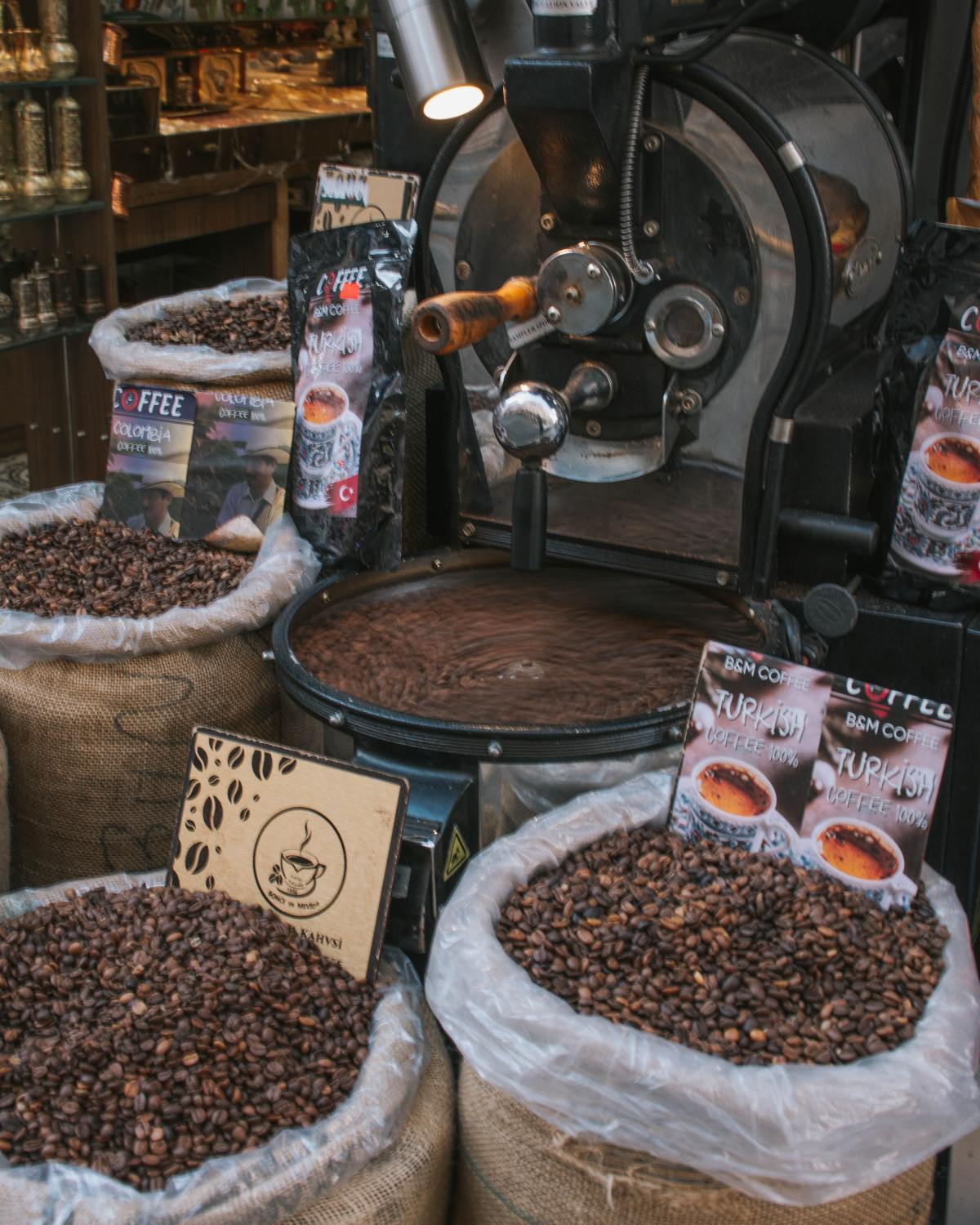
Problem description: The problem is to analyze coffee production trends by country over time and identify any patterns or insights in the data.
Related work: This problem is related to previous visual analytics work that has been done to analyze trends in agricultural production, such as crop yields and exports. One example of an existing visual analytics tool that addresses this is the Food and Agriculture Organization of the United Nations (FAO) Crop Production Dashboard. This image is the source of my inspiration, it mimics the nature of my project in commodity research. However, I wanted to expand upon it by making an animated version that can show changes happening over time so potential trends could be gleamed more intuitively.
Solution: To solve the problem of analyzing coffee production trends, we used an animated bar chart to show how coffee production has changed by country over time. We used the gganimate package in R to create the animation, which allowed us to easily transition between years and visualize the changes in coffee production. We also used the position_dodge() function to separate the bars for each year, making it easier to compare production levels across countries. Additionally, we used annotations and labels to provide additional information and context for the data, such as the Crop_year value and the country names.
In terms of methodology, we used a time series analysis approach to examine how coffee production has changed over time. By animating the bar chart, we were able to see how production levels have fluctuated over the years and identify any trends or patterns in the data. We also used a part-to-whole approach by showing how each country’s production level contributes to the total global production.
Overall, the use of an animated bar chart allowed us to effectively analyze and communicate trends in coffee production over time. This methodology can also be applied to other types of agricultural production data to identify patterns and insights in the data.
The data shows that Brazil is the largest coffee producing country in the world, with production increasing steadily from 2000 to 2010, then remaining relatively stable until 2017. Colombia, Vietnam, and Indonesia are also major coffee producers, with production increasing significantly over the past two decades.
However, some countries have experienced declines in coffee production. For example, production in Ethiopia, the birthplace of coffee, has decreased since the early 2000s. Similarly, production in Mexico and Peru has also declined over the past decade.
One interesting trend that emerges from the data is the increasing diversification of coffee production. In the past, Arabica coffee was the dominant variety, accounting for more than two-thirds of global production. However, over the past decade, the share of Robusta coffee has increased significantly, particularly in Vietnam, where it now accounts for more than 90% of coffee production.
The data also shows that coffee consumption is closely linked to coffee production. Countries that produce the most coffee also tend to consume the most. For example, Brazil, Colombia, and Vietnam are among the top coffee consuming countries in the world.
The Groundhog Day celebration in a town near Punxsutawney, Philadephia is a popular folk tradition that locals use as a fun way to predict the weather. As legend goes, if Punxsutawney Phil does not see his own shadow on the second day of February then an early spring is in store. Otherwise, if Punxsutawney Phil does see his own shadow then six more weeks of winter is to be expected.
Everybody knows that a groundhog may not be the best means we have in predicting the weather, but to what degree of certainty do we know that Punxsutawney Phil is a decent meteorologist? Well lucky for us, weather data is pretty simple to collect and in this case extensively documented. In this analysis of whether or not a groundhog can replace your local meteorologist, data obtained from the Punxsutawney Groundhog Club as well as the local weather records which goes back to 1898 will be sampled and used.
H₀: There is no significant correlation between Punxsutawney’s Phil seeing a full shadow and the coming of a long winter.
H₁: There is a significant correlation between Punxsutawney’s Phil seeing a full shadow and the coming of a long winter.
Below is the data collection and munging process. The file I used happened to be stored as a csv file which I later imported into my working environment RStudio, then I needed to remove blank fields and noise so the quality of the analysis is not compromised and skewed by empty or unclear variables. I also decided to remove unnecessary regions in the dataset, and in Punxsutawney Phil’s defence he is a Pennsylvania local and including data from the other regions of the United States just seems unnecessary when predicting local weather.
data <- read.csv(“groundhog_dataset.csv”, header = TRUE) data <- data %>% drop_na() data <- data %>% select(-3, -4, -5,-6, -7, -8, -9) data <- data %>% filter(!grepl(‘No Record’, Punxsutawney.Phil)) %>% filter(!grepl(‘Partial Shadow’, Punxsutawney.Phil)) #filter(!grepl(‘No Shadow’, Punxsutawney.Phil)) #%>% #filter(March.Average.Temperature..Pennsylvania. <= 32) data <- data[-c(116), ]
data
## Year Punxsutawney.Phil March.Average.Temperature..Pennsylvania. ## 1 1898 Full Shadow 42.0 ## 2 1900 Full Shadow 29.3 ## 3 1901 Full Shadow 35.1 ## 4 1903 Full Shadow 44.5 ## 5 1904 Full Shadow 34.0 ## 6 1905 Full Shadow 36.9 ## 7 1906 Full Shadow 29.1 ## 8 1907 Full Shadow 39.5 ## 9 1908 Full Shadow 38.4 ## 10 1909 Full Shadow 33.1 ## 11 1910 Full Shadow 42.6 ## 12 1911 Full Shadow 32.8 ## 13 1912 Full Shadow 31.5 ## 14 1913 Full Shadow 40.0 ## 15 1914 Full Shadow 31.7 ## 16 1915 Full Shadow 30.3 ## 17 1916 Full Shadow 28.2 ## 18 1917 Full Shadow 35.4 ## 19 1918 Full Shadow 39.3 ## 20 1919 Full Shadow 38.6 ## 21 1920 Full Shadow 36.7 ## 22 1921 Full Shadow 45.4 ## 23 1922 Full Shadow 37.1 ## 24 1923 Full Shadow 34.3 ## 25 1924 Full Shadow 33.5 ## 26 1925 Full Shadow 38.1 ## 27 1926 Full Shadow 30.2 ## 28 1927 Full Shadow 39.2 ## 29 1928 Full Shadow 34.0 ## 30 1929 Full Shadow 41.0 ## 31 1930 Full Shadow 35.1 ## 32 1931 Full Shadow 33.7 ## 33 1932 Full Shadow 30.8 ## 34 1933 Full Shadow 33.8 ## 35 1934 No Shadow 32.1 ## 36 1935 Full Shadow 40.0 ## 37 1936 Full Shadow 39.4 ## 38 1937 Full Shadow 31.4 ## 39 1938 Full Shadow 40.1 ## 40 1939 Full Shadow 35.6 ## 41 1940 Full Shadow 29.5 ## 42 1941 Full Shadow 28.9 ## 43 1944 Full Shadow 32.7 ## 44 1945 Full Shadow 46.2 ## 45 1946 Full Shadow 45.3 ## 46 1947 Full Shadow 30.3 ## 47 1948 Full Shadow 38.3 ## 48 1949 Full Shadow 36.8 ## 49 1950 No Shadow 30.8 ## 50 1951 Full Shadow 36.1 ## 51 1952 Full Shadow 34.6 ## 52 1953 Full Shadow 37.9 ## 53 1954 Full Shadow 35.0 ## 54 1955 Full Shadow 37.2 ## 55 1956 Full Shadow 32.9 ## 56 1957 Full Shadow 36.1 ## 57 1958 Full Shadow 33.7 ## 58 1959 Full Shadow 34.1 ## 59 1960 Full Shadow 24.5 ## 60 1961 Full Shadow 37.1 ## 61 1962 Full Shadow 34.2 ## 62 1963 Full Shadow 37.5 ## 63 1964 Full Shadow 36.9 ## 64 1965 Full Shadow 32.1 ## 65 1966 Full Shadow 37.5 ## 66 1967 Full Shadow 34.4 ## 67 1968 Full Shadow 38.4 ## 68 1969 Full Shadow 32.7 ## 69 1970 No Shadow 31.6 ## 70 1971 Full Shadow 32.5 ## 71 1972 Full Shadow 33.1 ## 72 1973 Full Shadow 42.9 ## 73 1974 Full Shadow 36.9 ## 74 1975 No Shadow 33.7 ## 75 1976 Full Shadow 40.8 ## 76 1977 Full Shadow 41.2 ## 77 1978 Full Shadow 31.9 ## 78 1979 Full Shadow 39.4 ## 79 1980 Full Shadow 33.3 ## 80 1981 Full Shadow 34.1 ## 81 1982 Full Shadow 34.9 ## 82 1983 No Shadow 38.7 ## 83 1984 Full Shadow 29.5 ## 84 1985 Full Shadow 38.3 ## 85 1986 No Shadow 38.0 ## 86 1987 Full Shadow 39.0 ## 87 1988 No Shadow 37.2 ## 88 1989 Full Shadow 36.7 ## 89 1990 No Shadow 40.2 ## 90 1991 Full Shadow 39.5 ## 91 1992 Full Shadow 34.5 ## 92 1993 Full Shadow 32.8 ## 93 1994 Full Shadow 33.8 ## 94 1995 No Shadow 39.7 ## 95 1996 Full Shadow 31.8 ## 96 1997 No Shadow 37.6 ## 97 1998 Full Shadow 39.7 ## 98 1999 No Shadow 34.2 ## 99 2000 Full Shadow 42.6 ## 100 2001 Full Shadow 33.3 ## 101 2002 Full Shadow 38.2 ## 102 2003 Full Shadow 37.2 ## 103 2004 Full Shadow 39.5 ## 104 2005 Full Shadow 32.3 ## 105 2006 Full Shadow 37.0 ## 106 2007 No Shadow 37.4 ## 107 2008 Full Shadow 35.6 ## 108 2009 Full Shadow 38.2 ## 109 2010 Full Shadow 42.0 ## 110 2011 No Shadow 36.3 ## 111 2012 Full Shadow 47.7 ## 112 2013 No Shadow 33.9 ## 113 2014 Full Shadow 30.3 ## 114 2015 Full Shadow 31.6 ## 115 2016 No Shadow 43.4
And now onto some exploratory analysis
summary(data)
## Year Punxsutawney.Phil March.Average.Temperature..Pennsylvania. ## Length:115 Length:115 Min. :24.50 ## Class :character Class :character 1st Qu.:33.00 ## Mode :character Mode :character Median :36.10 ## Mean :36.00 ## 3rd Qu.:38.65 ## Max. :47.70
Here we find that the average temperature across the many years sampled in March lie around 36 degrees Fahrenheit. But to better visualize this I have made a graph that tracks the average March temperatures split between the observations of a full shadow(orange) and no shadow (cyan).
Notice the spread of the shaded area wrapping around our models of linear regression. This goes to show how little correlation exists between whether our groundhog saw its shadow or not and whether a longer winter or an early spring are due. There does seem to be vaguely a pattern of warmer average temperatures when the groundhog does not see his own shadow. However, this can be attributed to the smaller sample size of the occurrence of a no shadow, relative to a full shadow with a sample size of 100 and 15 for no shadow. The difference in sample sizes skews the different averages a bit.
And now we explore the validity of whether or not Punxsutawney’s Phil has a knack in weather prediction or not. And I will be doing this with a linear regression model, putting Punxsutawney’s Phil observation of a full shadow or no shadow as the predictor variable and the recorded temperature averages as the explanatory variable. Below is the code that does exactly that.
data_regression <- lm(data$March.Average.Temperature..Pennsylvania. ~ data$Punxsutawney.Phil, data = data) summary(data_regression)
## ## Call: ## lm(formula = data$March.Average.Temperature..Pennsylvania. ~ ## data$Punxsutawney.Phil, data = data) ## ## Residuals: ## Min 1Q Median 3Q Max ## -11.447 -2.947 -0.020 2.553 11.753 ## ## Coefficients: ## Estimate Std. Error t value Pr(>|t|) ## (Intercept) 35.9470 0.4245 84.689 <2e-16 *** ## data$Punxsutawney.PhilNo Shadow 0.3730 1.1753 0.317 0.752 ## — ## Signif. codes: 0 ‘***’ 0.001 ‘**’ 0.01 ‘*’ 0.05 ‘.’ 0.1 ‘ ‘ 1 ## ## Residual standard error: 4.245 on 113 degrees of freedom ## Multiple R-squared: 0.0008906, Adjusted R-squared: -0.007951 ## F-statistic: 0.1007 on 1 and 113 DF, p-value: 0.7515
Unfortunately, after looking at the negative adjusted R-squared values and the p-value which sits above 0.7 the prospects of our little groundhog reliably predicting the arrival of an early spring or a longer winter is just very low.
Conclusion
A P-value of 0.7515 denotes that we have failed to reject the null hypothesis, meaning that there is a great degree of chance involved in the measured outcomes displayed in the graph above. Which sadly, makes our little groundhog an unreliable meteorologist and that we should just stick to the weather channel instead for our weather forecasts.